Data Readiness, RAG Engineering and Context Engineering: A Field Guide

Most RAG projects do not fail on the model. They fail on a PDF parsed into soup, on a chunk that lost its section title, on a filter applied after the search instead of inside it, on a context window filled to 90 % because nobody measured where it starts to degrade. This guide walks the whole chain in the order the data flows through it, and for each step gives the mechanism, the parameters that matter, the failure mode, and the criterion that decides.

It condenses a 49-slide working deck I wrote for an enterprise data and AI team. The original list of topics had two columns, "data readiness and RAG engineering" on one side and "context engineering" on the other. Here they are reorganised as seven steps, because the two columns are one pipeline: the first four steps produce candidate passages, the last two decide what actually enters the model.

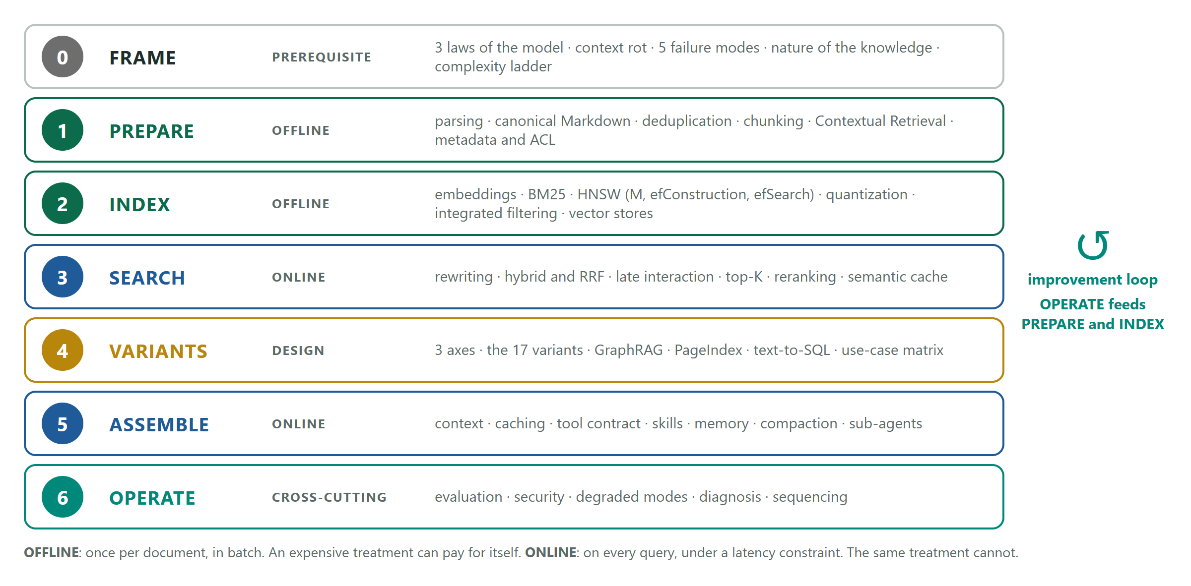
One distinction structures every trade-off in what follows. Offline work happens once per document, in batch: an expensive treatment can pay for itself. Online work happens on every query, under a latency constraint: the same treatment cannot. The loop on the right of the figure matters too: evaluation at the OPERATE step feeds back into parsing and indexing. It is the loop most projects forget to draw.

Step 0. Frame before you build

Nothing technical yet. Three laws of the model, five failure modes of the context, and two framing questions that decide the architecture before any tooling.

Law 1: a model has no memory, only an input

A language model is a stateless function. A sequence of tokens goes in, a sequence comes out, and between two calls nothing survives. What we call "the conversation" is a reconstruction on the application side: at every call, the whole history is sent again, billed again, and it occupies the window at the expense of everything else.

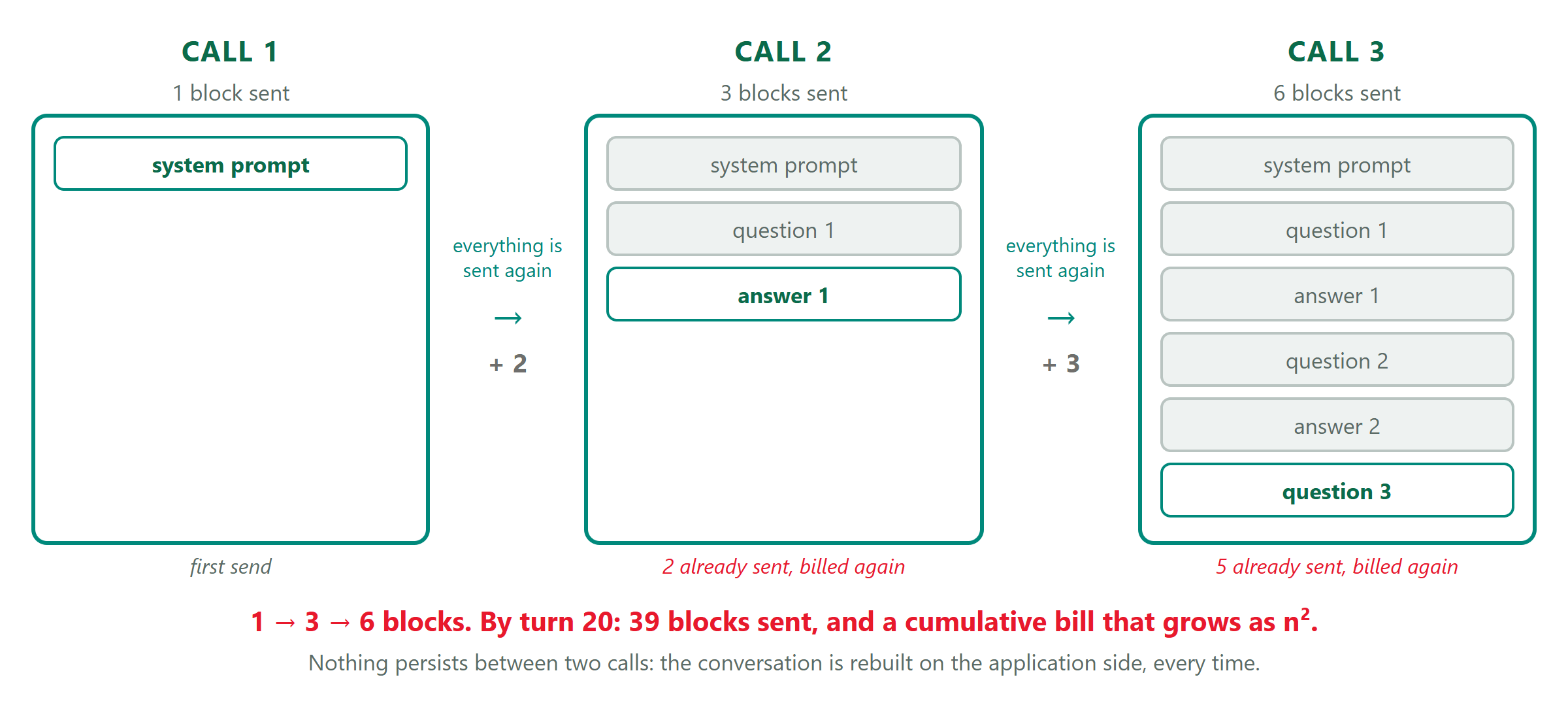
The consequence is the only question that matters in this whole guide: which tokens enter the context? Steps 1 to 4 (prepare, index, search, variants) produce candidates. Steps 5 and 6 (assemble, operate) choose what goes in. A persistent memory is application state, never model state.

Law 2: the context degrades before it is full

Degradation precedes overflow, and it has been measured. Chroma Research tested 18 models on 1M-token contexts in July 2025: reliability breaks between 300k and 400k tokens, the degradation depends on the similarity between the question and the passages rather than on length alone, and beyond a few thousand words even a plain copy task starts to fail.

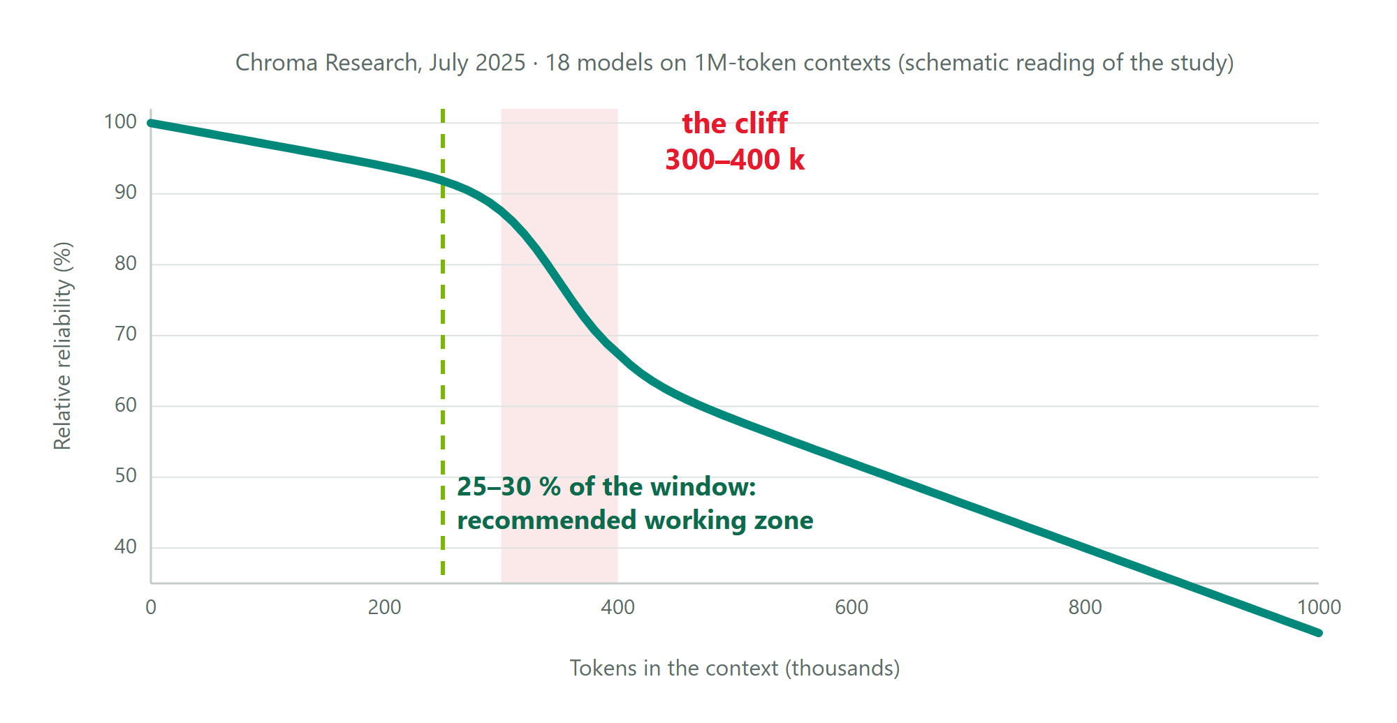
The sizing rule that follows: the RULER benchmark puts the truly usable context at 50 to 65 % of the advertised window. In production, aim for 25 to 30 %, and measure before extending.

The second result is the most structuring fact in this guide. Liu et al. (TACL 2024) placed the relevant passage at different positions among 20 passages passed to GPT-3.5-Turbo.

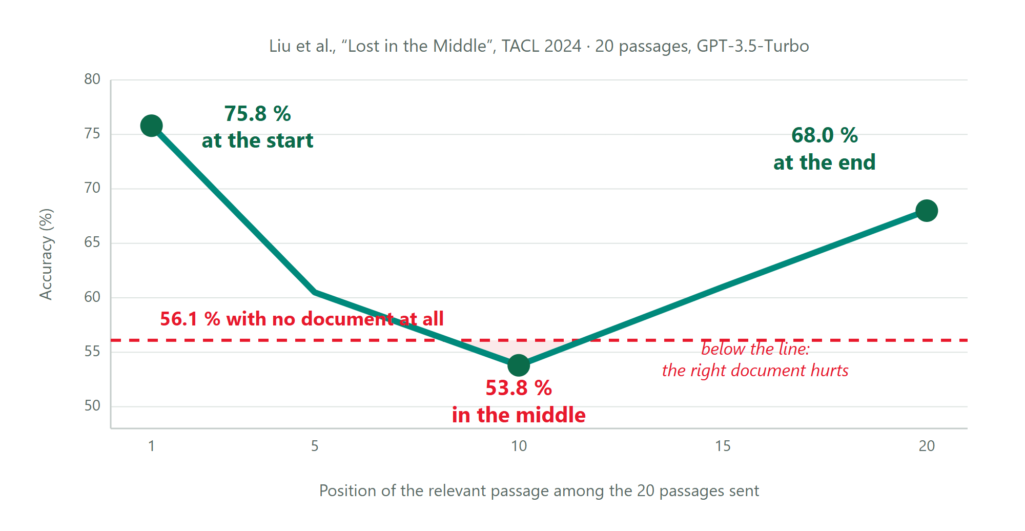
At the start, 75.8 % accuracy. In the middle, 53.8 %. With no document at all, the model scores 56.1 %. In the middle of the context, providing the right document produces a worse result than providing nothing. The context can become a liability.

The five failure modes of the context

Naming the failure mode is what lets you choose the remedy. Each one has a distinct treatment, and applying the wrong diagnosis applies the wrong fix.

Failure	Mechanism	Concrete example	Remedy
Lost in the middle	The start and the end are processed better than the middle: a U-shaped curve	The right document is at position 14 of 25 and gets ignored	Order the passages · reduce K
Distraction	Moderately relevant content drowns the relevant content	20 chunks with 2 useful ones do worse than 3 chunks with 2 useful ones	Selection · score threshold · pruning
Tool confusion	More declared tools, lower selection rate	60 MCP tools plugged in: it calls the wrong one, or loops	Tool search · a lean tool contract
Conflict (versions, freshness)	Two contradictory pieces of information coexist in the context	v1 and v2 of a procedure come back together	Freshness metadata · purge
Poisoning	An error written into the context is re-read as a fact	A hallucination at turn 3 becomes a truth at turn 12	Selective compaction · isolation through sub-agents

These five lines are the diagnostic grid reused at the OPERATE step: faced with a wrong answer, identify which failure is in play. The rule underneath: the context is a budget, not storage. Past a certain fill level, adding information degrades the answer.

Two framing questions before choosing an architecture

The first question is what kind of knowledge has to be mobilised. Two lines out of five do not call for a RAG at all.

What kind of knowledge?	The tool, and why
Figures, aggregates, current states	Text-to-SQL or an API call. A model must never add up what it has read.
Large volumes of documentary facts, to be cited	RAG. This is the rest of the guide.
Know-how, a procedure, a format	Skills: versioned files loaded in tiers.
A behaviour, a tone, a protocol	System prompt, and fine-tuning if the volume justifies it. Fine-tuning learns a style, never recent facts.
A small, stable, heavily consulted corpus	Long context or CAG: searching would cost more than reading. Threshold: the three cumulative conditions in step 4.

The second question is which step of the complexity ladder to stop at.

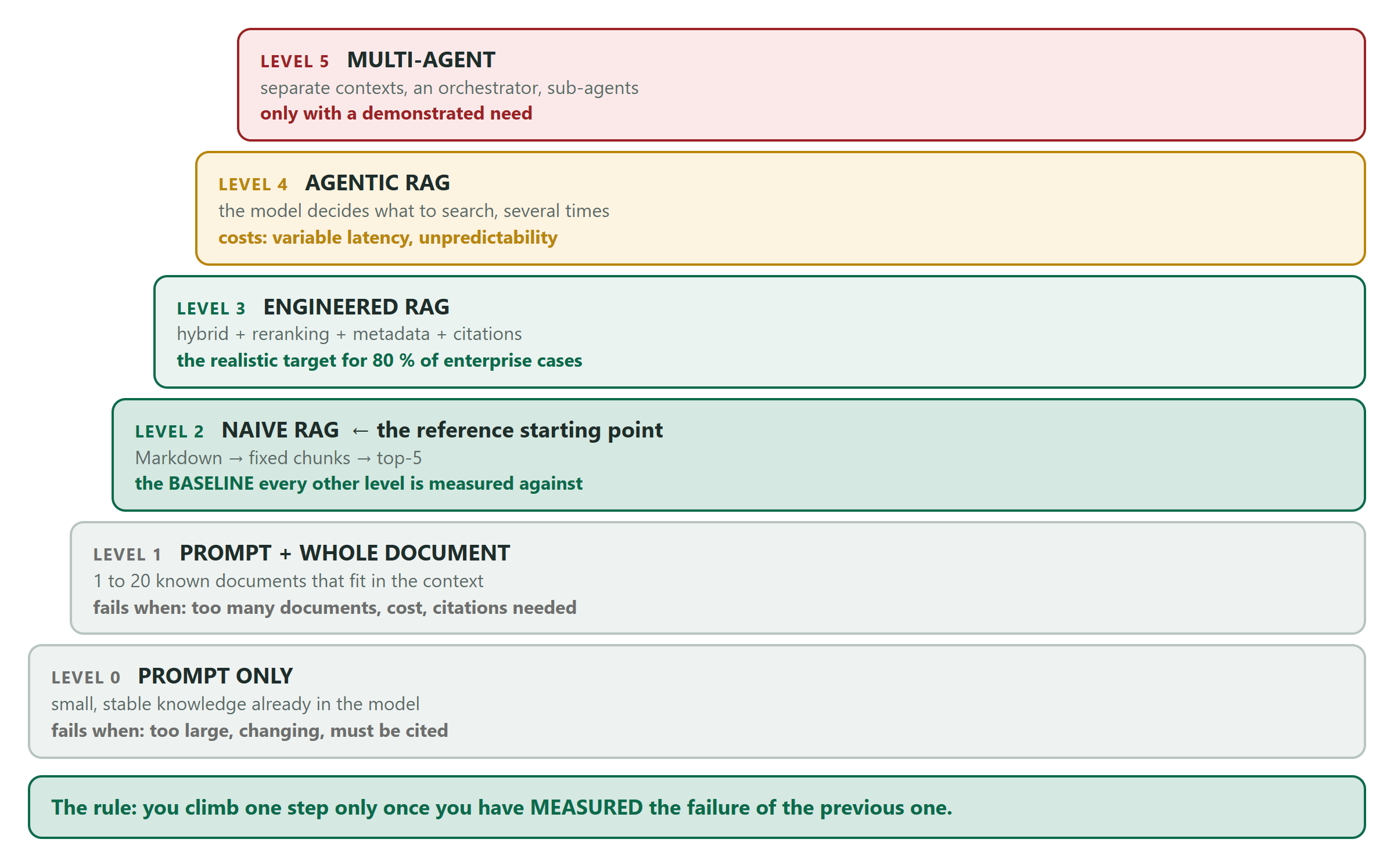
The rule of ascent: you climb one step only once you have measured the failure of the previous one. The most frequent mistake is to start at level 4 because everyone is talking about it. Level 1, prompt plus whole document, is almost always skipped although it requires no infrastructure at all.

And a third law, which fixes the order of everything that follows. Law 3: information lost at parsing is never recovered downstream. And the failure is silent: the answer is well written, and wrong.

The reference architecture

Now that the constraints are set, here is the architecture that follows from them. Every box in this map answers one of the three laws or one of the five failures.

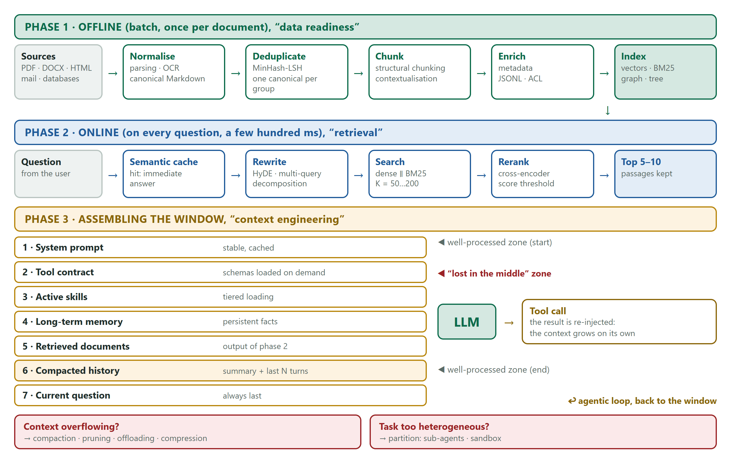
Three tiers, with a different cost of error at each:

• Phase 1, offline, once per document. An error here lowers the quality ceiling for everything downstream.
• Phase 2, online, on every question. An error here means the right passage never reaches the model.
• Phase 3, assembling the window. An error here means the passage is present but badly exploited.

Security and access rights are not a phase: they cut across all three. Handled downstream, they read as content filtering. They are an architecture decision, and they appear as five rules in the map:

1. Phase 1: access-control lists are carried by the chunk, never reconstituted after the fact.
2. Phase 2: filtering is integrated into the query. With post-filtering, unauthorised content enters the context before being discarded.
3. Phase 2: the semantic cache is partitioned per tenant, with document identifiers in the key.
4. Phase 3: every retrieved piece of content is data, never an instruction.
5. Phase 3: the model proposes an action, a deterministic component validates it: real permissions, schema, ceilings, log.

The review criterion fits in three questions: on which sensitive data does the system operate, to which uncontrolled content is it exposed, and what capacity to emit outward does it retain? This is the "lethal trifecta" (Simon Willison): remove any one of the three conditions and the exfiltration path closes.

One nuance on phase 3: compaction and the construction of long-term memory are semi-offline. They do not carry the latency constraint of the rest of the phase.

Step 1. Prepare the data

Everything here is offline, so an expensive treatment can be worth it. Law 3 fixes the order: what is lost at parsing is not recovered.

The canonical document

A PDF is a list of rendering instructions. It contains no paragraphs, no reading order, no tables in the computing sense. A heading is a heading only by its visual attributes.

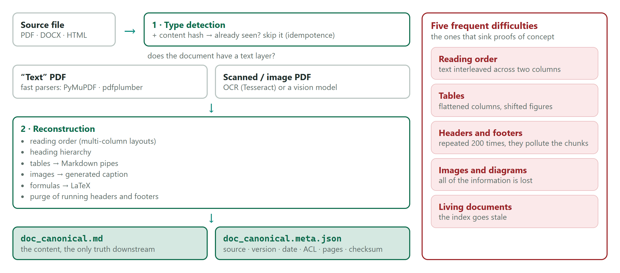
Why canonical Markdown: the structure becomes explicit and machine-readable, which is what makes structural chunking, hierarchy and section trees possible. The markup is economical (about 3 tokens against 12 in HTML), the format is heavily present in training data, and it is plain text, therefore versionable and auditable.

Two artefacts, not one: the canonical document, and a metadata descriptor that includes the section-to-page mapping. Without the descriptor there is no citation, no filtering by rights, no incremental reindexing. Throwing it away forces you to re-parse everything later. For reindexing: a content hash to detect changes, a document version and an effective date to retire superseded versions. Dense tables (balance sheets, risk matrices) keep their CSV or JSON source next to the Markdown.

Two approaches to the conversion itself: a modular pipeline, or a vision model. The difference that matters is not the benchmark score but the failure mode. A pipeline fails visibly. A vision model can invent plausible content. Route by source type.

Chunking: the trade-off, and how to sidestep it

Every chunking is constrained from both sides: a single vector for two hundred pages no longer discriminates, and the whole document does not fit in the budget. The two qualities move in opposite directions.

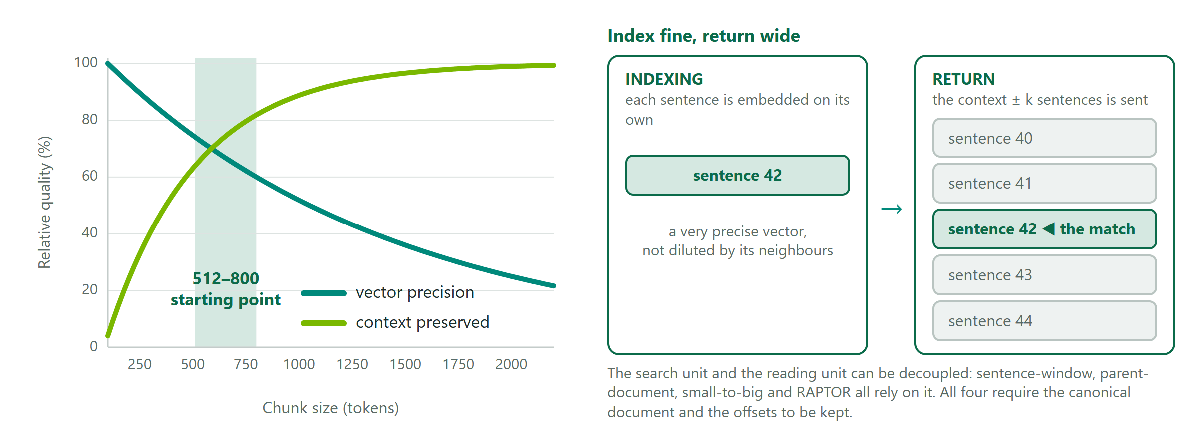
The way around the trade-off is to separate the search unit from the reading unit: index fine, return wide. Six strategies, by increasing cost: fixed size, recursive, structural (the right default as soon as normalisation is reliable), semantic (one embedding per sentence, very variable size), late chunking (encode the document, then split the vectors), agentic. The marginal gain decreases fast: the gap from fixed to structural exceeds the gap from structural to agentic.

The constraint to decide on day one: sentence-window, parent-document, small-to-big and RAPTOR all require keeping the canonical document and the offsets in the metadata. A pipeline that keeps only detached chunks forbids these approaches; adopting them later means re-parsing everything.

Starting point: 512 to 800 tokens, 10 to 15 % overlap. The optimum depends on the density of the corpus, the window of the embedding model and the maximum context of the reranker. These three choices are decided together, not separately.

Contextual Retrieval: the cumulative effect

A chunk pulled out of its document loses its references. "The ceiling is raised to 15 % beyond the threshold of the previous paragraph": no query can match this chunk, and it stays unreadable even when found. The fix is to prefix each chunk with 50 to 100 tokens of generated context before indexing.

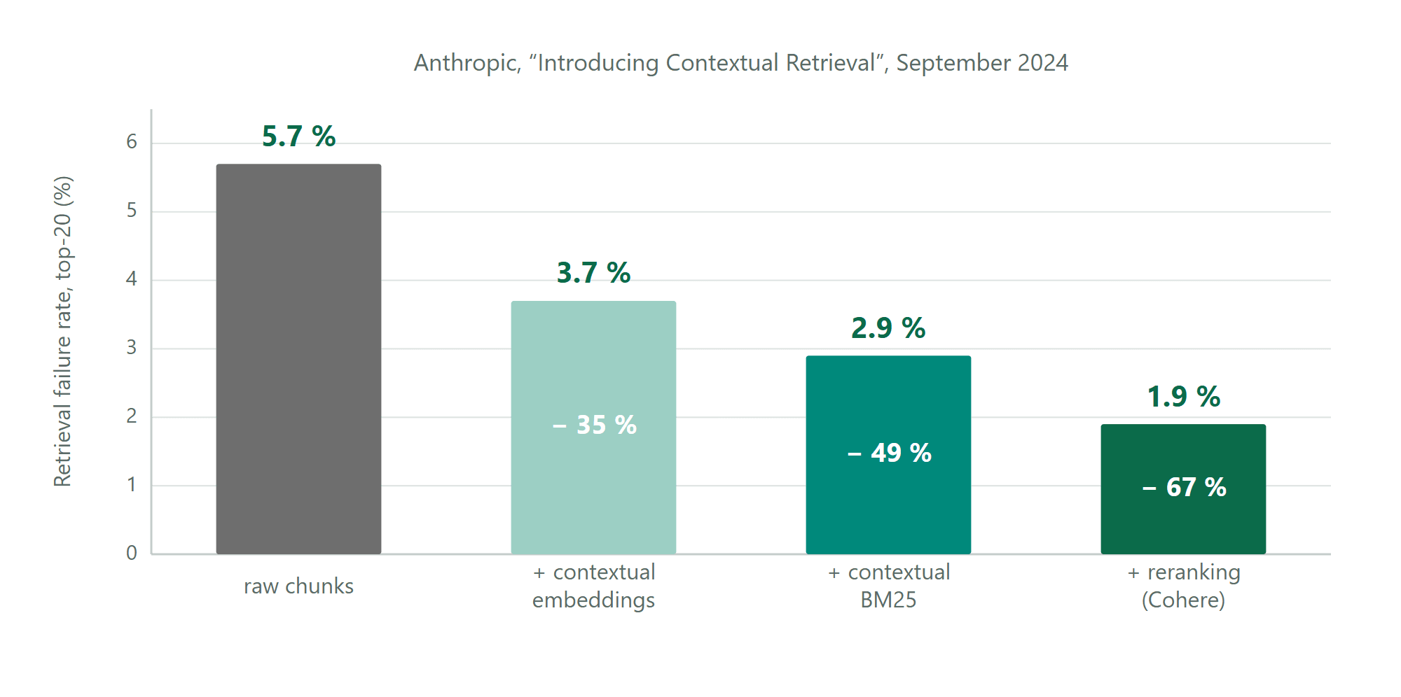
Anthropic's results (September 2024): 5.7 % failure at baseline, 3.7 % with contextualisation, 2.9 % adding the lexical index, 1.9 % with reranking, a 67 % reduction in total. The point to remember is not the final figure but the shape of the curve: the gains are cumulative, and no single technique is sufficient alone. This pattern repeats throughout the guide.

The cost is one LLM call per chunk at indexing, made acceptable by prompt caching (around $1 per million tokens). Without caching the approach is not economical. It is the cache that makes it accessible, not the technique itself.

Two complementary enrichments come almost free. The breadcrumb ("Quality manual > 4.2 > 4.2.3") costs nothing: normalisation already produced it. Hypothetical questions, generated and indexed offline, align the index with the shape of real queries. Same goal as HyDE, but the cost is paid once.

The chunk is a record, and the corpus must be deduplicated

A chunk carries an identity, an origin, rights and a temporal validity.

{
  "chunk_id":        "doc_4f2a1c#s12#c003",
  "doc_id":          "doc_4f2a1c",
  "source_uri":      "sharepoint://HR/CBA-2024.pdf",
  "doc_version":     "2024-06-01",
  "content_hash":    "sha256:9ab3...",
  "section_path":    ["Title III", "Article 12"],
  "page_start":      47,
  "offset_start":    18422,
  "effective_date":  "2024-01-01",
  "acl":             ["group:HR", "group:management"],
  "embedding_model": "bge-m3@1.0",
  "dedup_group":     "grp_88c1",
  "context_prefix":  "...",
  "text":            "..."
}

Field	What it does
acl	Filter applied inside the query, never after
source_uri + page	Without a citation there is no verifiability, therefore no adoption
version + hash	Incremental reindexing, idempotent reruns
effective_date	Discriminate superseded versions: compliance
offset_start	Technical precondition for sentence windows
embedding_model	Identifies what to reindex if the model changes
dedup_group	Discard duplicates at query time

Deduplication, often absent from pipelines, produces the most visible symptom on the business side: the engine returns two contradictory procedures because the same manual exists in four versions across three repositories, and it returns the most similar one, not the most current. Four levels: exact hash of the text, MinHash-LSH, vector similarity, redundancy filtering at query time. Nothing gets deleted: one canonical is designated per group. And an ordering note: deduplication runs before chunking, as the architecture map shows. Deduplicating after chunking means processing the same document four times.

The storage format is JSONL, one JSON object per line: stream processing, append by concatenation, corrupted lines isolated, easy parallelisation, readable diffs. The five industrialisation properties of the pipeline: idempotent, resumable, incremental, versioned, deployable without downtime (index v2 built alongside, reversible switch).

Of everything in this step, access control carried by the chunk is the one thing impossible to fix after the fact.

Step 2. Index and make it findable

Two complementary representations, seven index families, and the hard point projects discover late: filtering by rights.

Represent, then search fast

Representation	Mechanism	What to know
Dense (embeddings)	Projection into a space where proximity approximates meaning	What gets lost first is the rare: references, acronyms, codes
Matryoshka	Signal concentrated on the first dimensions	Truncation 3,072 → 512 with bounded loss: memory divided by 6
Lexical (BM25)	IDF, saturation (k1 = 1.2), length normalisation (b = 0.75)	BM25F weights title, body and summary separately
Language analysers	Lucene analysers: elisions, accents, stemming	In hybrid, use light stemming: aggressive stemming creates false positives
Learned sparse (SPLADE-v3)	Sparse vector with automatic term expansion	Lexical exactness plus semantic coverage. Non-commercial licence, so permissive alternatives: BGE-M3 (sparse head), OpenSearch neural sparse

Dense covers synonymy but loses the rare; lexical does the opposite; learned sparse tries to unite the two.

Seven index families: Flat, IVF, HNSW, IVF-PQ, ScaNN, DiskANN, SPANN. Implementations: pgvector, OpenSearch, Qdrant, Elasticsearch. The industry default is HNSW, and it has three parameters, only one of which is tuned live:

• M (default 16) drives recall and memory; fixed at creation. On Pinecone's SIFT1M measurement, moving M from 2 to 512 takes the index from about 0.5 GB to about 5 GB: a factor of 10 on a single parameter.
• efConstruction improves the graph without touching latency; fixed too.
• efSearch trades recall against latency and is tuned live: it is the operations parameter.

Two thresholds that save engineering: below about 50,000 vectors, exact search is enough (100 % recall, nothing to tune). DiskANN moves the cost from RAM to SSD and makes billions of vectors affordable. For sizing: 5M vectors × 1,024 dimensions × 4 bytes × 1.4 ≈ 29 GB in float32. A reference point: 100M vectors in 1,536 dimensions ≈ 600 GB before the index structure.

Choosing the family comes down to three questions in order: volume, then memory, then latency.

Question	Answer
Fewer than 50,000 vectors	Flat, exact search. 100 % recall, no parameter, nothing to rebuild
50k to 50M, RAM is enough	HNSW in float32, M = 16, efConstruction = 200
50k to 50M, RAM is not enough	HNSW + quantization, scalar or binary, with oversampling ×3 to ×4 and rescoring on the full vectors
More than 50M, latency under 50 ms required	IVF-PQ or ScaNN. Aggressive in-memory compression: the recall is measured, never assumed
More than 50M, latency tolerant	DiskANN or SPANN. The cost moves from RAM to SSD

Two cross-cutting constraints whatever the node reached: binary quantization is never used without rescoring, and the engine must produce a correct top-k with a filter that excludes 99 % of the corpus.

Quantize, and filter by rights

Quantization is the most profitable cost lever, on one condition.

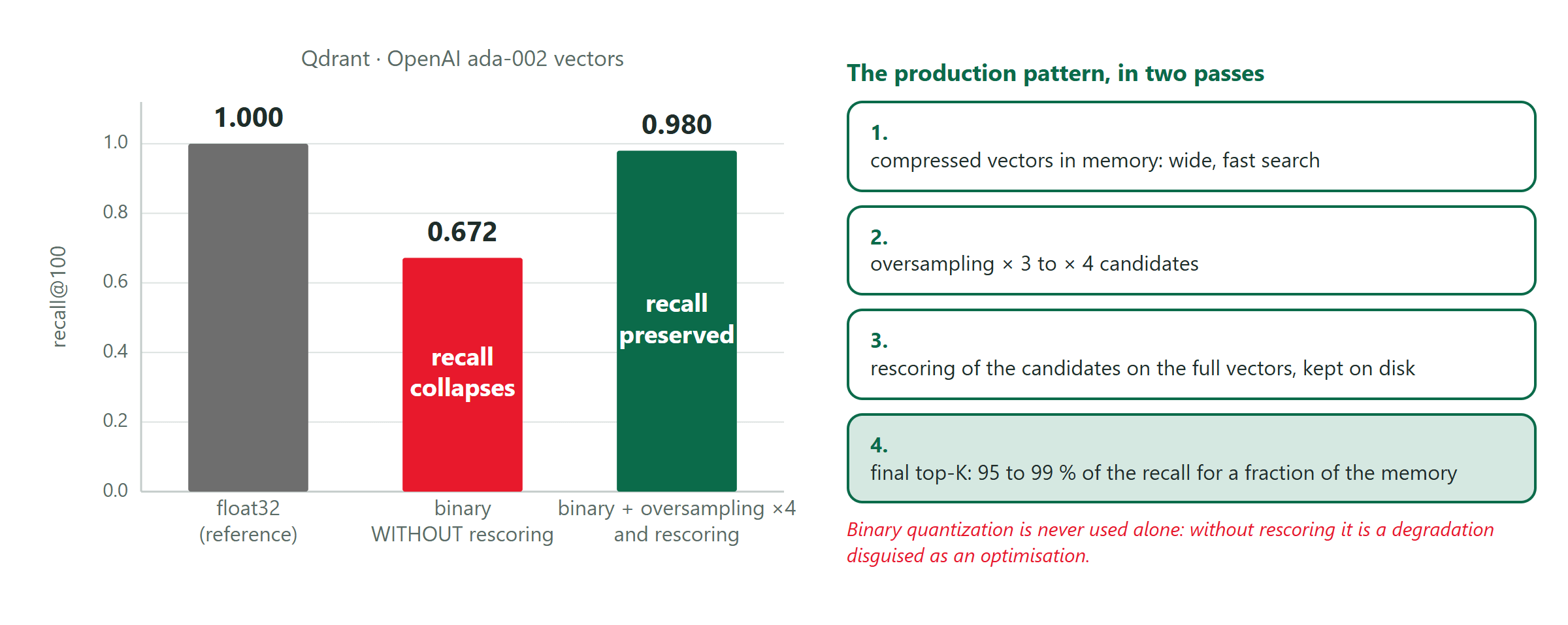
In binary without rescoring, recall falls to 0.672. With oversampling and rescoring it climbs back to 0.98. This is not a tuning option, it is the condition of use. The production pattern in two passes: compressed vectors in memory for a wide, fast search; oversampling ×3 to ×4; rescoring of the candidates on the full vectors kept on disk; final top-K. It restores 95 to 99 % of the recall for a fraction of the memory.

Filtering is the point that blocks production launches. The real query is never "the k nearest" but "the k nearest within the authorised subset". Three strategies, two of which fail:

• Post-filtering. Search, then filter. With a selective filter the result can be empty while relevant, authorised documents exist. Worse: unauthorised content can enter the context before being discarded. An empty result is visible; this leak is silent.
• Pre-filtering. Search within the subset. But the graph was built on the whole set: removing nodes from it degrades its navigation.
• Integrated filtering. The condition is evaluated during the graph traversal. The only approach that preserves both recall and rights.

The selection criterion for an engine follows directly: can it produce a correct top-k with a filter that excludes 99 % of the corpus?

Step 3. Search, then rank

We move online: every decision is paid in latency on every query. Miss nothing first, then bring the best to the top.

The query pipeline and its latency budget

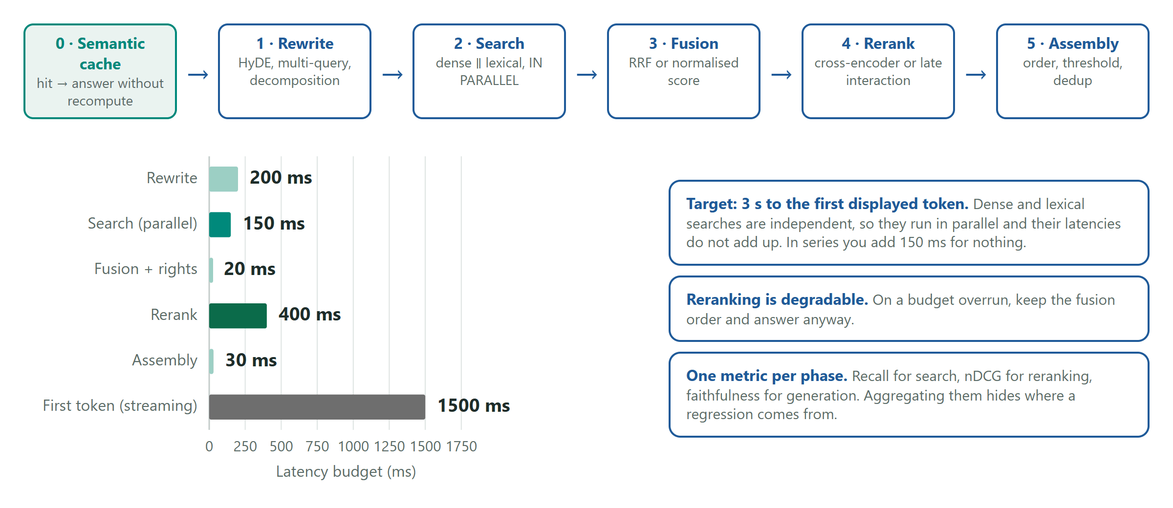
Five phases, each with its own metric and its own behaviour on overrun: rewriting (HyDE, multi-query, decomposition), search (dense and lexical in parallel), fusion (RRF or normalised score), reranking (cross-encoder or late interaction), assembly (order, threshold, deduplication). The target is 3 seconds to the first displayed token.

Two properties of the pipeline are exploitable. The dense and lexical searches are independent: run in parallel, their latencies do not add up. In series, you add 150 ms for nothing. And reranking is degradable: on overrun, keep the order from the fusion and answer anyway. One metric per phase: recall for search, nDCG for reranking, faithfulness for generation. Aggregating them prevents you from locating a regression.

The semantic cache is one more phase, upstream of all the others. If an equivalent question has already been handled, the answer is returned without recomputation. Observed hit rates: 30 to 70 % on FAQ-type traffic, much lower on agentic traffic where the queries are generated and therefore more varied. But a badly partitioned cache has already returned one customer's data to another. Four rules: partition per tenant, include the document identifiers in the key, start at a similarity threshold of 0.97, exclude amounts and dates. Streaming does not reduce total latency, only the time to the first token, which is what the user perceives.

Fuse dense and lexical

The two methods have disjoint failure profiles. This is not an arbitration, it is a composition.

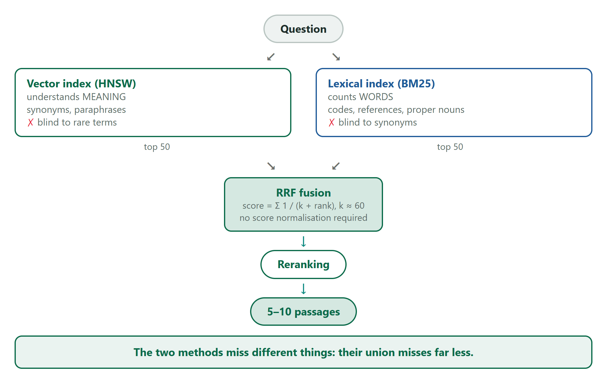
The line that often decides: on vocabulary never seen in training (a project name, a product code), dense would require retraining. Lexical works immediately. In an enterprise this is decisive: at the launch of a project with new terms, only lexical answers.

Why reciprocal rank fusion (RRF) rather than a weighted sum: the scores are not comparable. BM25 is unbounded, cosine is bounded, and a weighted sum requires a normalisation that drifts with the corpus. RRF uses only ranks: no parameter to calibrate, and it extends to any number of lists. Default k = 60 (Cormack et al., SIGIR 2009). Native in Elasticsearch, Azure AI Search, MongoDB Atlas and Weaviate.

Late interaction: the moment of the meeting

Three regimes, distinguished by the moment at which the question and the document interact.

Regime	Encoding	Score	Profile	Scale
No interaction (bi-encoder)	Q → 1 vector, D → 1 vector	cos(q, d)	very fast · average precision · minimal storage	billions of documents
Late interaction	Q → n vectors, D → m vectors	MaxSim(Q, D)	fast (precomputable) · good precision · heavy storage	millions of documents
Full interaction (cross-encoder)	Q and D read together by the model	f(Q, D)	slow · maximum precision · no storage	tens of documents

"Late" names the moment of the meeting. In a cross-encoder it happens at the entrance of the network, hence the precision and the impossibility of precomputing. In late interaction each side is encoded separately and the meeting is deferred to an arithmetic operation: for each token of the question, keep the best match in the document, then sum. The property that counts is that absence is penalised. A document with no term close to "fibre" loses points, where a single vector would have drowned that gap in the average.

Costs: ColBERTv2 stores 20 to 36 bytes per vector instead of 256, an MS MARCO index of 16 to 25 GB instead of 154, at 50 to 250 ms latency. PLAID divides further, up to ×7. ColPali applies the principle to page images: no OCR, no chunking. But with no extracted text there is no lexical index and no literal citation. Storage is 50 to 200× the dense baseline in raw form, brought down to 2 to 4× with 2-bit quantization. That figure is what decides adoption.

Calibrate top-K, then rerank

Two stages, two jobs: a wide, cheap recall stage, then an expensive precision stage.

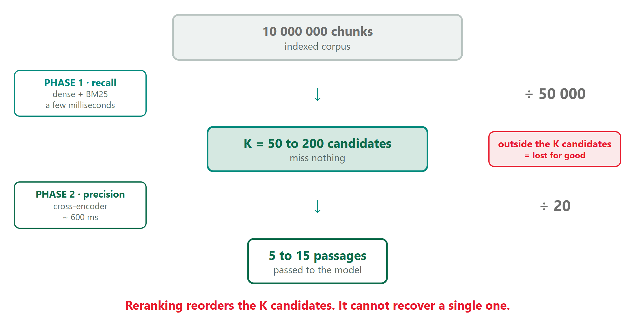
The structuring property: a passage absent from the K candidates is lost for good, and the failure is silent. A K that is too small produces no error. The system answers on worse passages, without any alert. Only a golden set reveals it. If K is capped by latency, act on recall upstream (hybrid, chunking) rather than reranking harder.

The diagnostic rule: if the reranker does not move nDCG, the problem is recall, not ranking. Act on chunking, embeddings or the hybrid setup. For scale, Voyage's rerank-2 on nDCG@10 moves FinanceBench from 0.80 to 0.91 (+14 %) and MultiHiertt from 0.25 to 0.46 (+84 %). The offer: Cohere Rerank (about 600 ms, multilingual), Voyage (specialised), BGE-reranker (self-hosted), ColBERT as a second stage. A generalist reranker underperforms on a highly specialised corpus: legal, medical, financial.

The bi-encoder compares two summaries. The cross-encoder judges "does this document answer the question?": more precise, but not precomputable. Hence the two stages.

Step 4. Choose the architecture

We enter this step through the business question, not the catalogue. In a third of use cases, the answer is not a RAG.

Translate a business need into an architecture

Start with the case where a RAG is the wrong tool.

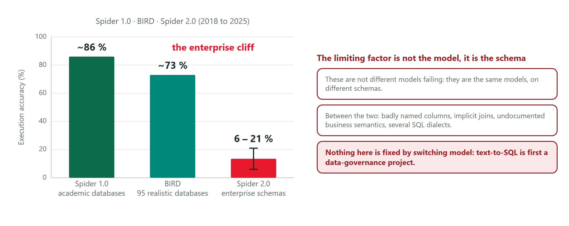
The limiting factor is not the model, it is the schema. These are the same models scoring 86 % on Spider 1.0, 73 % on BIRD, and 6 to 21 % on Spider 2.0 with enterprise schemas of more than three thousand columns. Between the two: badly named columns, implicit joins, undocumented business semantics, several SQL dialects. Nothing here is fixed by switching model. Text-to-SQL is first a data-governance project.

The matrix from need to architecture, which is the synthesis of the first four steps:

Use case	Architecture	Index	Decisive reason
Internal FAQ, level-1 support	Hybrid + rerank + answer cache	Vector + BM25	Volume, latency, stable corpus
Long financial reports	PageIndex / vectorless	Section tree	Similarity is not relevance
Supplier risk	GraphRAG for routing + vector	Graph + vectors	Multi-hop questions
Steering, KPIs	Text-to-SQL	Relational warehouse	Exactness of the figures
Internal procedures	Skills	Versioned files	Procedural need
Code repository	Agent + file tools	None	Freshness beats latency
A 30-page knowledge base	CAG	None	Searching costs more than reading

Four of these seven lines call for no RAG at all.

Cache-augmented generation (CAG, Chan et al., 2024) preloads the whole corpus and caches the KV state. No search, therefore no retrieval failure. Three cumulative conditions: the corpus fits in 25 to 30 % of the context; it is stable, since one modified document invalidates the whole cache (exact prefix, see prompt caching below); and everyone is allowed to see everything, since the cache is shared without ACL. One "no" and it is a RAG.

The most common framing error: choosing a RAG variant before checking that a RAG is the right answer.

Three axes and seventeen variants

The names that circulate do not describe mutually exclusive alternatives. They are positions on three independent axes:

1. What is represented in the index? A chunk, a sentence, a hierarchy of summaries, an entity graph, a section tree, token multi-vectors, image patches, table rows.
2. What is the relevance signal? Dense, lexical (BM25), hybrid, late interaction, LLM reasoning, a SQL query.
3. Who drives the loop, and how many times? A single fixed pass, self-evaluation plus correction, adaptive routing, an agentic loop, several agents.

Reading examples: GraphRAG = entity graph · dense plus summaries · local/global routing. PageIndex = section tree · LLM reasoning · navigation loop.

The seventeen variants, in four groups, with their maturity. The directory is not a list of projects, it is a qualification grid: which group does a proposal belong to, and do we actually have the corresponding constraint?

#	Name	What it solves	Maturity
1 to 5 · The maturation continuum, the normal trajectory of a project
1	Naive RAG	The starting point, the measurement baseline	Standard
2	Advanced RAG	Most of the failures of naive RAG	Standard
3	Modular RAG	Industrialisation, testability	Standard
4	Hybrid RAG	Rare terms, references, acronyms	Standard
5	Hierarchical (RAPTOR)	Broad questions	Production
6 to 8 · A corpus constraint: visual, made of linked entities, or long and structured
6	Multi-vector (ColBERT, ColPali)	Fine-grained matches, visual documents	Production
7	Graph RAG	Multi-hop, global questions	Production
8	Vectorless (PageIndex)	Long structured documents, traceability	Experimental
9 to 13 · A question constraint: routing, correction or chaining
9	Adaptive RAG	Complexity engaged only when it helps	Production
10	Corrective RAG (CRAG)	Incomplete corpora, out-of-scope queries	Experimental
11	Self-RAG	Hallucinations, useless retrievals	Experimental
12	Agentic RAG	Multi-step questions, actions	Production
13	Multi-agent RAG	Exploration volume, parallelism	Experimental
14 to 17 · Outside textual RAG: the reference data is not text, or fits in the context
14	Multimodal RAG	Visual corpora	Production
15	Structured / Text-to-SQL	Figures, aggregates, exactness	Standard
16	RAFT	Robustness to retrieval noise	Experimental
17	CAG	Small, stable corpora, zero latency	Production

The maturity column is for prioritising. An experimental proposal is not disqualified, it requires a pilot and a stopping criterion.

The decision tree asks four questions, in order. The first three leave RAG entirely; only the fourth chooses a variant.

1. What is the nature of the reference data? Figures, aggregates, exactness → Structured / Text-to-SQL, not a textual RAG. Visual documents, forms, drawings → Multimodal RAG, ColPali.
2. Does the corpus fit in the context? Yes, small, stable, everyone entitled → CAG, preloading and prefix caching, no search.
3. Is what is missing knowledge or behaviour? A behaviour, a tone, a format → RAFT or fine-tuning, not a retrieval problem.
4. Which constraint dominates? The corpus (rare terms, linked entities, long documents) → Hybrid, RAPTOR, ColBERT, Graph RAG, PageIndex. The question (routing, correction, chaining) → Adaptive, CRAG, Self-RAG, Agentic, Multi-agent. No particular constraint → Naive RAG, then Advanced, then Modular: the maturation continuum.

The graph: what it solves and what it costs

Two classes of question escape passage retrieval: multi-hop questions whose answer exists in no single document, and global questions that bear on the corpus as a whole. The graph pipeline: entity and relation extraction by LLM, entity resolution ("Dupont Ltd" = "DUPONT SA"), community detection (Leiden), one summary per community. Entity resolution is a data-quality problem, not an AI problem, and it is always underestimated. The graph also requires an ontology, which is business work done beforehand.

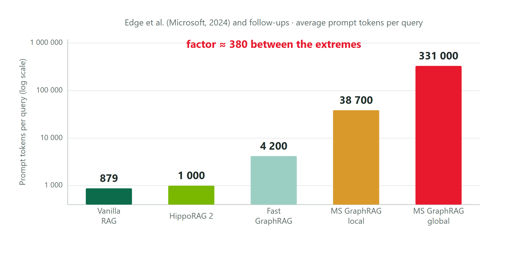
The cost, to be announced frankly: one LLM call per chunk of the entire corpus, difficult incremental updates, and at query time a factor of about 380 between vanilla RAG and Microsoft's global mode.

Two ways not to pay it. LazyGraphRAG (Microsoft, 2025) indexes at the cost of vector RAG, about 0.1 % of full GraphRAG, and builds the graph on demand; neighbours are LightRAG, HippoRAG 2, Fast GraphRAG. And above all, the document graph rather than the entity graph: edges derived from the citations already produced at the PREPARE step, for a marginal cost. The recommended route: the graph as a routing layer, vectors to retrieve the text. Never as the only engine.

Vectorless: replace similarity with navigation

This approach removes similarity search instead of improving it. A tree of sections is built with a summary at each node, and the model walks it.

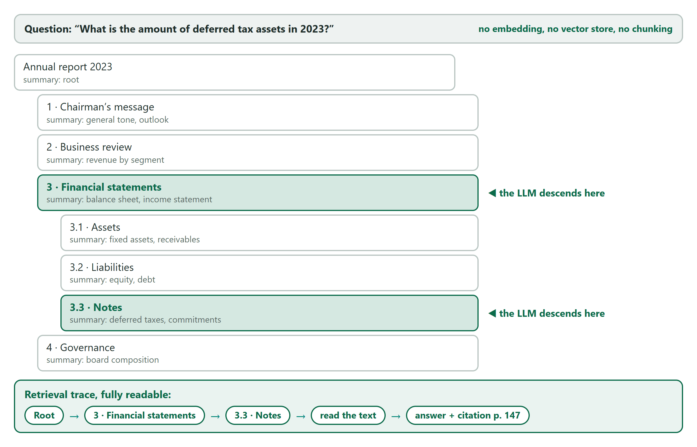
Four things vectors do not handle:

1. Similarity is not relevance. In a long document, the passage closest to the question is often the introduction, which reuses its vocabulary, not the appendix that contains the figure.
2. Internal cross-references. "See appendix G" has no similarity with its target.
3. Arbitrary chunking disappears, replaced by the editorial structure.
4. The navigation path is a native explanation trace, which counts in an auditable context.

What it costs: several model calls per query, so several seconds, and a cost out of proportion with a vector search. And a total dependence on the quality of the tree, therefore on the PREPARE step. A message thread has no table of contents.

The balance point: an indexing cost is traded for a per-query cost. Vector search amortises at indexing; the tree indexes almost nothing. It depends on the ratio of queries to documents: at high query volume, vector search becomes preferable again. The logic is the same as the just-in-time regime of the next step: give a map and tools, rather than preloading everything by similarity.

Step 5. Assemble the context

The objective inverts. Until now we tried to miss nothing. Now we look for the smallest set of tokens that is sufficient. This is the most developed step of the guide, because it is where decisions get made daily once the RAG is in place.

The context is no longer written, it accumulates

In a conversational application you write a prompt and get an answer: the context is fixed, written by hand, and the required skill is to formulate. In an agentic system every tool call re-injects its result: the context grows without anyone writing it, and the required skill is to arbitrate.

Curation is four operations, in this order:

1. Select: which information enters.
2. Order: at the start and the end, not in the middle.
3. Format: a compact table, not verbose JSON. The same information serialised one way or the other varies by a factor of three, and this is a lossless optimisation.
4. Prune: remove what has already been exploited.

The order is imposed: pruning before ordering destroys the ranking. The operational criterion: every block present in the context must justify its place by an expected contribution to the answer. A context is not storage, it is an allocation under constraint.

The confusion to avoid is between "memory" and "full history". Replaying the whole history is only accumulation, and it triggers all five failures from the framing step. Memory is an act of selection, not of conservation.

The anatomy of the context

Seven zones, from the most stable to the most volatile, and their order has two direct technical consequences.

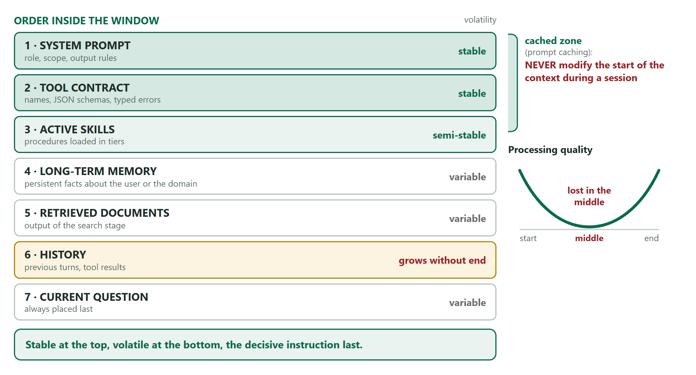
Consequence 1: the cache works on an exact prefix. Placing the stable material first lets it be billed at the reduced rate. Corollary: never modify the start of the context during a session. A timestamp at the top or a reordered tool list invalidates the cache at every call, a cost regression that is hard to spot.

Consequence 2: position influences processing. The decisive instruction last, the documents before the question: the question is read in the light of the documents. On five passages, the most relevant first and the key element recalled just before the question. The two extremities are the best processed.

Zone 6, the history, is the only one that grows without bound. Everything else in this step is about managing it.

Prompt caching

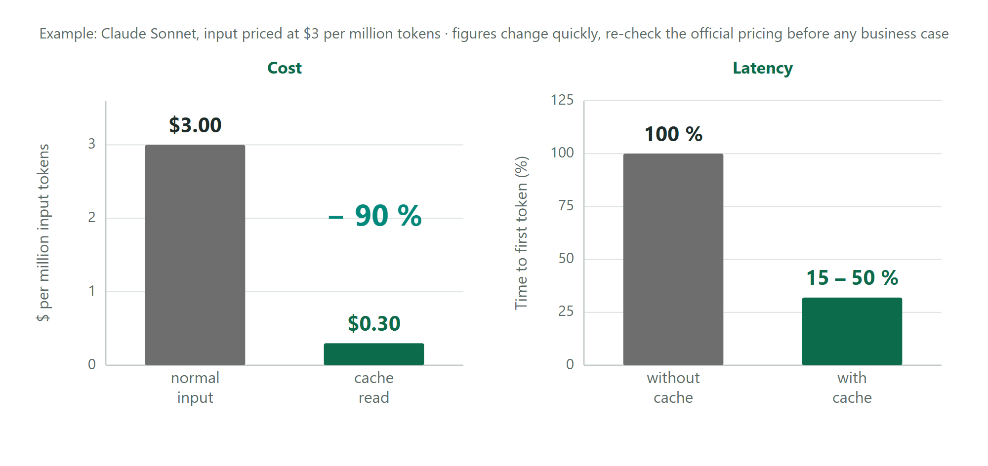
The only mechanism in this guide that acts on cost and latency at the same time, with no counterpart in quality.

Provider	Cache read	Conditions
Anthropic	0.1× (−90 %)	Threshold around 1,024 tokens, profitable from the first re-read
OpenAI	−50 to −90 %	Automatic, writes not billed
Google	Explicit or implicit (−75 %)	Explicit beyond 32k tokens

A model at $3 per million input tokens drops to 30 cents on cache reads, and the time to first token falls by 50 to 85 %. The condition of use is prefix invariance: any change upstream invalidates the whole cache downstream. No timestamp at the top, no reordered tool list, no interpolated user name. This is what imposes the ordering discipline of the previous section.

The point often missed: the cache is what makes Contextual Retrieval viable in the PREPARE step, one call per chunk at indexing brought down to about $1 per million tokens. Prices change quickly. Re-check the official documentation before any business case.

The system prompt: a question of altitude

Two writing modes produce fragile systems, for opposite reasons.

Too specific: an accumulation of conditional rules covering particular cases. The behaviour becomes unmaintainable and fails outside the enumerated cases. It is business logic written in a medium with no typing and no tests.

Too generic: a role description with no operational constraint. "You are a helpful assistant who helps employees." The behaviour is neither predictable nor steerable, and no change is attributable.

The useful register is decision heuristics: precise enough to guide, general enough to cover the cases not foreseen. "If the question is about an amount, cite the source and the date of the applicable version; if the information is absent, say so instead of estimating."

The method of evolution: start from a minimal prompt, and add a rule only in response to an observed failure, never by anticipation. Version it and regression-test it, like code. It sits in zone 1: modifying it during a session invalidates the cache. Form matters as much as substance: tagged sections, one idea per section, zero redundancy, since two formulations of the same rule create ambiguity. The minimum of information that produces the intended behaviour, written to be maintained by a human in six months. A system prompt is a software component: versioned, tested, reviewed. Not a text adjusted as you go.

The tool contract, and the hidden cost of tools

For the model, a tool exists only through its description. An ambiguous interface produces a failing agent.

Element	Good practice	Counter-example	Consequence
Name	Verb + object: search_customer_contract	get_data · tool3 · query	The model guesses
Description	What it does, when to use it AND when not to	"Searches data"	Overlapping scopes
Parameters	Typed, allowed values enumerated, examples	filters: object	Malformed calls in a loop
Errors	Typed and actionable: expected format YYYY-MM-DD	Error 500 · Bad request	The agent loops instead of correcting

The applicable test: would a developer discovering the set know how to choose without hesitation from the descriptions alone? If not, neither will the model.

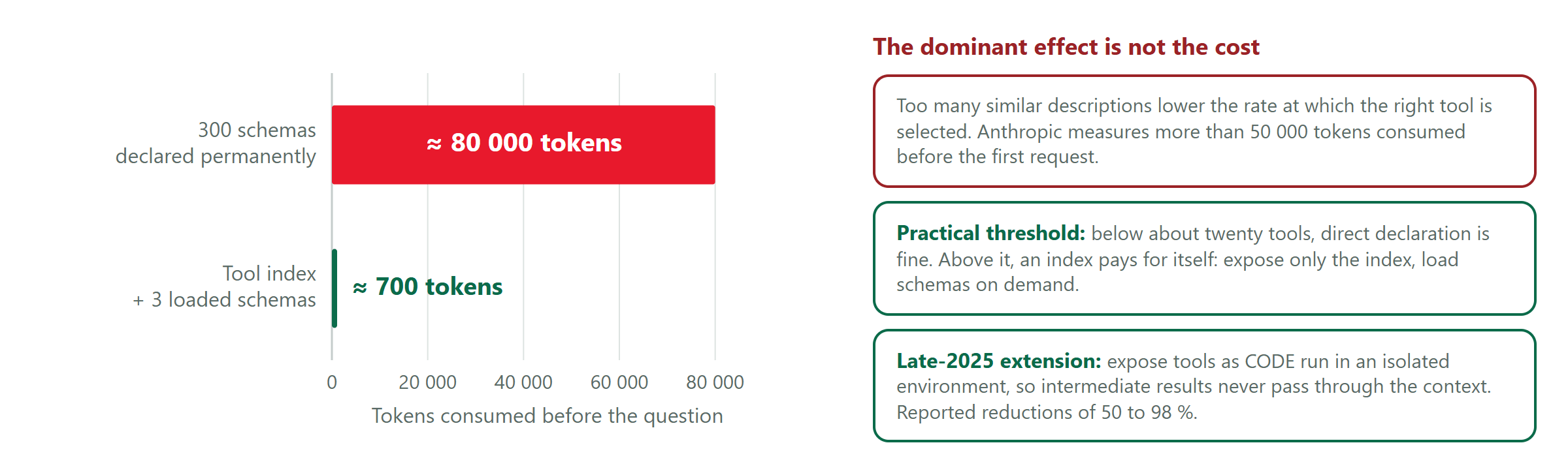
The dominant effect is not the cost. Too many similar descriptions lower the rate at which the right tool is selected. Anthropic measures more than 50,000 tokens consumed before the first request. The answer reuses the pattern of the SEARCH step: expose only an index, load the schemas on demand. The practical threshold: below about twenty tools, direct declaration is enough. Above it, the index pays for itself. A late-2025 extension exposes tools as code executed in an isolated environment, so that intermediate results no longer pass through the context at all, with reported reductions of 50 to 98 %.

Skills: procedural knowledge in tiers

An organisation's know-how cannot be maintained in a system prompt. It would represent hundreds of thousands of tokens, almost all of them off-topic for any given request.

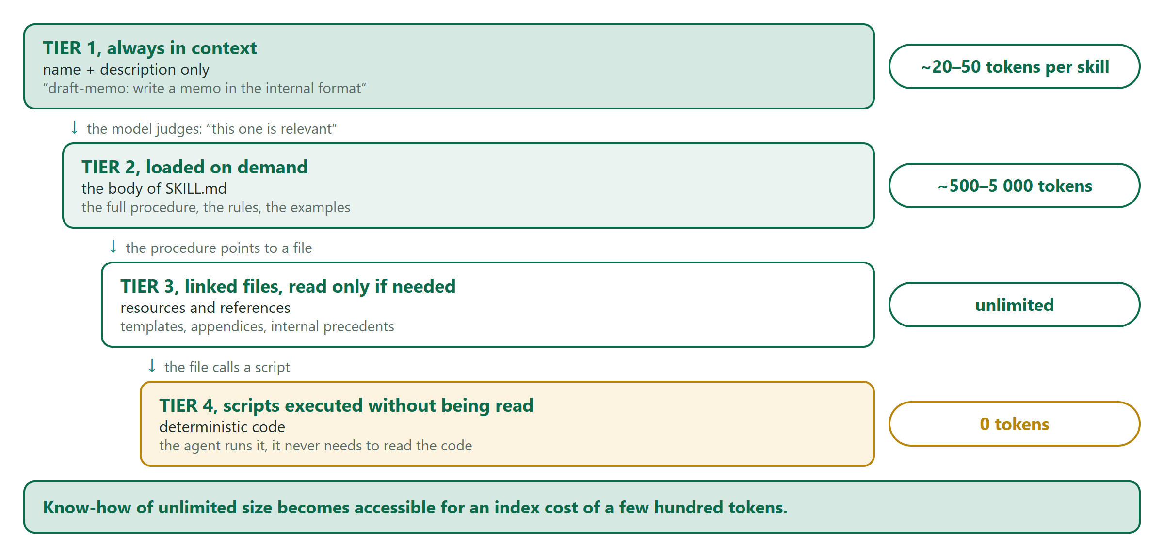
Loading happens in tiers: name and description permanently, the procedure on demand, resources if the procedure points to them, and scripts executed without being read. Tier 4 is the most interesting architecturally: deterministic logic returns to tested code instead of being simulated by the model, at zero token cost. The capitalisation mechanism: know-how of unlimited size for a few hundred tokens of index, and a versioned folder instead of instructions duplicated across ten prompts. The total volume is unlimited; only tier 1, a few dozen tokens per skill, stays permanently in context.

Who fetches the information: two regimes

The central question of the step, and the hinge with everything before it.

Criterion	Pre-inference (push)	Just-in-time (pull)
Principle	"I guess what it will need and give it in advance": question → RAG → 10 passages → LLM, one round trip, everything decided before the model reasons	"I give it a map and tools, it goes and looks": list the folder, open this file, answer, N round trips, minimal context
Latency	Low, predictable	High, variable
Cost	Controlled	Variable
Context consumed	Fixed, useful or not	Minimal
Freshness	What was indexed	The data at time T
Progressive discovery	One chance to guess	The agent refines along the way
Predictability, audit	High	Every run differs

What really distinguishes the two regimes is not the volume but the moment of the retrieval decision. Pre-inference: once, with no way back. Just-in-time: revised at every turn, at the price of an unbounded number of turns. What made the second regime practical: a reference costs far less than content. A file path says nature, date and subject in ten tokens. In practice a mixed architecture wins: a preloaded core to guarantee a relevant starting point, plus tools to explore beyond it. It is exactly the PageIndex pattern.

Memory beyond the session

Short-term memory lasts the session: the turn history, tool results, the current plan, the open files. It disappears at the end of the session, or earlier, at compaction. Long-term memory has three natures: episodic (what happened: "on 12 March we decided X"), semantic (facts: "the user works in legal"), procedural (know-how, which is exactly what skills are).

A memory system is four policies decided explicitly: write (what to memorise, when), read (what to reload at start-up), conflict (what to do when a new fact contradicts an old one), forget (lifetime, purge). The real subject is not the choice of tool but the definition of these policies. The absence of a conflict policy is what makes a memory dangerous over time: it accumulates incompatible facts and serves them all as authoritative. Zep handles obsolescence with a temporal graph in which every fact carries a validity interval.

The implementation to evaluate first: Markdown files that the agent reads and edits itself. Readable, correctable, versionable, auditable, no infrastructure. A very useful case is the handover note: at the end of a session the agent writes where it is, its decisions, what remains, and the traps. The next session starts by reading it. It is the minimum viable memory.

A warning on method: the same memory system has been scored at 84 %, 58.44 % and 75.14 % on LoCoMo depending on which party publishes the figure. These scores are usable as an indication of direction, never as a selection criterion.

When the context overflows: five mechanisms

By order of aggressiveness. Pruning is free and non-destructive: apply it first, always.

Mechanism	What it does	What it costs
Pruning	Remove whole blocks without transformation: tool results already exploited, duplicates, abandoned branches	Zero, non-destructive for the rest
Compression	Replace several turns with a summary	One model call, and a definitive loss of information
Compaction	Rebuild the context when a threshold is crossed (80 to 95 %)	The compaction prompt is a critical component
Offloading	Move the information out and keep only a reference	Makes long sessions possible
Prompt compression	A small model scores the informativeness of each token and prunes the least useful	LongLLMLingua: +21.4 % at about 4× fewer tokens

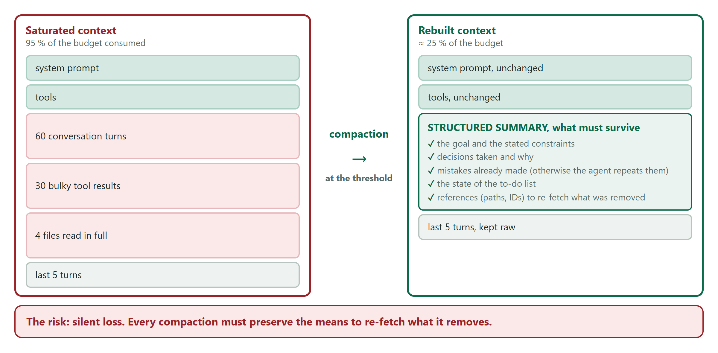
What the compaction must preserve: the goal and the stated constraints; the decisions taken and their justification; the mistakes already made, since without them the agent repeats them, which is the typical symptom of a badly specified compaction; the state of the task; and the references that allow re-fetching what was removed.

Prompt compression comes with three reservations that explain its low adoption: the compressor costs a model call, the result is hard to debug, and on structured content accuracy drops (text-to-SQL: 0.63 → 0.37). Stay extractive on code, SQL and tables. The risk common to all five mechanisms is unsignalled loss, because the agent does not know what was removed. Every compaction must keep the references.

Partition across several contexts

When a task exceeds the capacity of one context, the answer is no longer compression but partition.

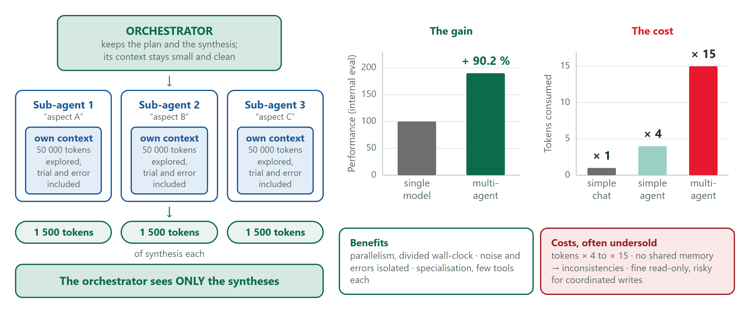
Anthropic's report (June 2025, Opus orchestrator with Sonnet sub-agents): +90.2 % on their internal evaluation, for fifteen times the token consumption. About 80 % of the performance variance is explained by token volume alone. The useful mechanism is the separation of exploration and synthesis: a sub-agent burns tens of thousands of tokens in trial and error and returns only about a thousand. The compression ratio matters as much as the parallelism, because the noise never reaches the orchestrator.

The validity domain is strict. Read-only and parallelisable: yes. Coordinated writes: risky, for lack of shared state. The sandbox variant: run a script rather than pass the data through the context, and the computation becomes exact. Real cost: ×4 to ×15 in tokens. Reserve it for high-value tasks, and measure rather than assume.

Step 6. Operate: evaluate, secure, diagnose

This step cuts across the six previous ones and closes the improvement loop. Without a golden set, no decision in the upstream steps can be arbitrated.

Measure: two levels not to aggregate

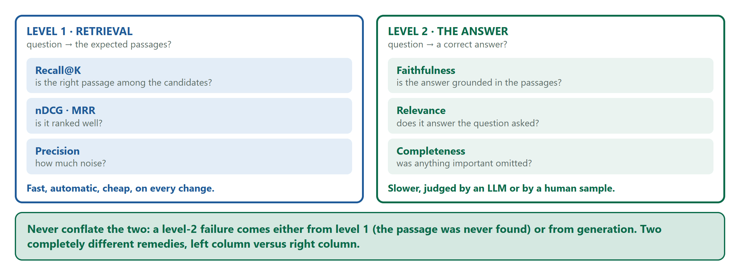
Level 1, retrieval: recall and nDCG, automatable, on every change. Level 2, the answer: faithfulness, relevance, completeness, judged by a model or by a human sample. They are never aggregated, for a diagnostic reason: a level-2 failure comes either from level 1 (the passage was never found) or from generation, and the fixes are disjoint.

The prerequisite is the golden set: 50 to 200 business questions with their expected passages, built with the users. It is what makes every previous decision arbitrable. To bootstrap it, generators (Ragas, DeepEval) produce question-context pairs from the corpus. But this silver set only becomes gold after human review.

The determining element of tracing: the final assembled context must be recorded and inspectable. It is the only piece of data that settles a diagnosis. Without it you can only formulate hypotheses. Standards: OpenTelemetry GenAI, Langfuse, Phoenix, LangSmith. Evaluation: RAGAS, DeepEval, TruLens, Giskard. Benchmarks: BEIR and MTEB for retrieval, FinanceBench and MultiHop-RAG for realism, CRAG and FRAMES end to end.

Secure: there is no native separation between code and data

In a context, the system instruction, the retrieved document and the tool result have the same status. Everything is text at the same level. Security consists of re-establishing the separation at the architecture level.

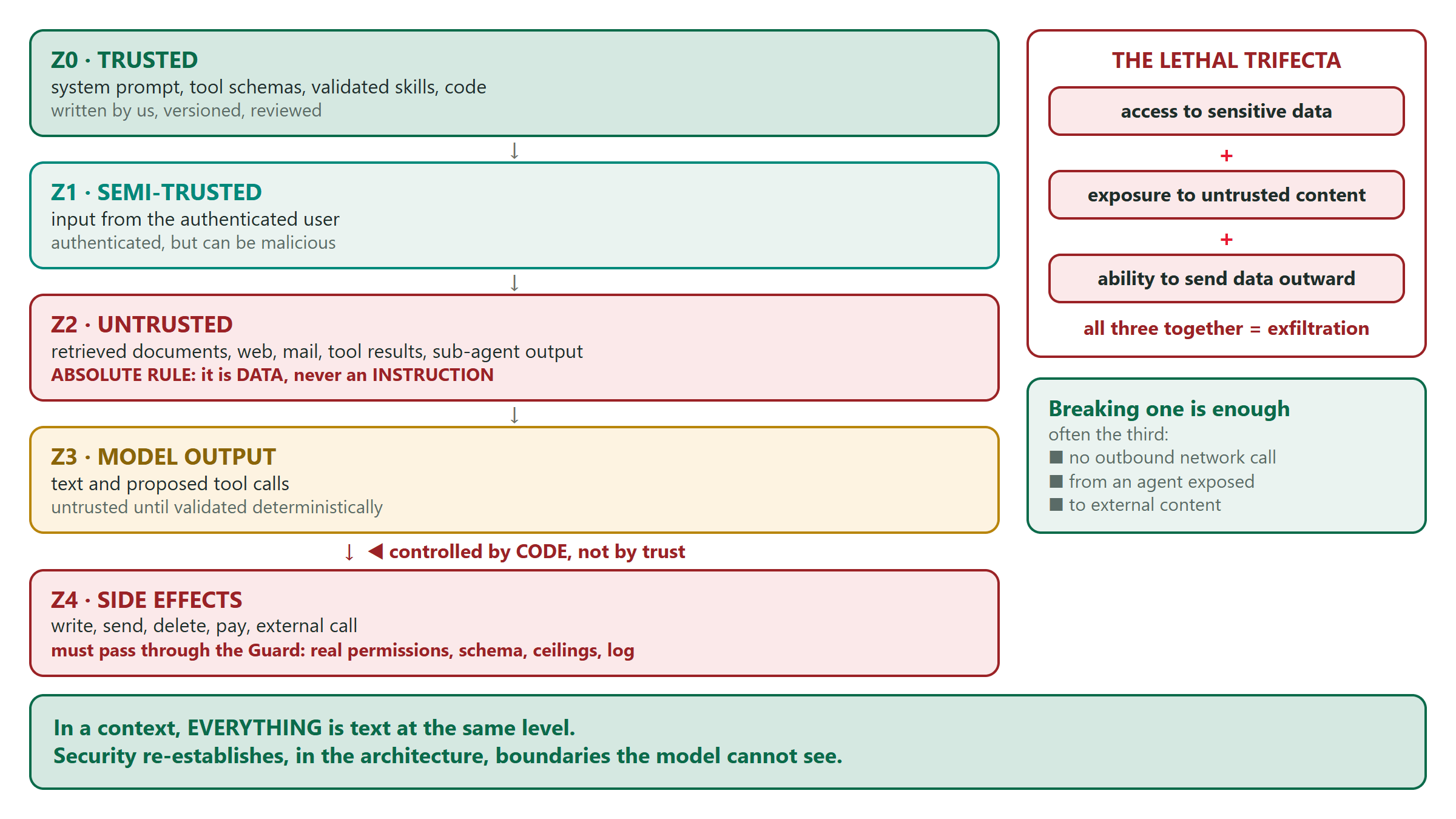
The central rule sits in zone 2: every retrieved piece of content is data, never an instruction. The model proposes an action; a deterministic component validates it against real permissions, a schema, ceilings and a log. What OWASP specifies: indirect injection is the number one risk, and it cannot be fully prevented. It is a property of the execution model, not a fixable bug. The answer is defence in depth, not a filter. The most operational criterion for a review is the trifecta: removing one of the three conditions closes the high-impact vector, and it is often the third, no outbound network call from an agent exposed to external content. Documented defences: CaMeL (Google DeepMind), "Design Patterns for Securing LLM Agents", least privilege, isolation, human review on anything irreversible.

Make it reliable: a system with no specified degraded mode has one by default

And its default degraded mode is hallucination.

Unavailable component	Degraded mode	Accepted loss
Embedding or vector index	Fall back to the lexical index	Synonym coverage; exact terms still work
Lexical index	Vector only	Exact references less reliable
Reranker over budget	Keep the fusion order	Lower top-5 precision
Main model	Fall back to a secondary model	Lower synthesis quality
No candidate above the threshold	No answer, with a suggestion	None: this is the expected behaviour

The last line is the most important. When no candidate passes the threshold, the expected answer is no answer. The functional loss is zero. A system that always answers is a system that fabricates an answer when it has none.

Retries and circuit breakers: replay only transient errors (429, 5xx, timeouts), never a validation error. Exponential backoff with jitter to desynchronise clients, a ceiling on attempts, then the degraded mode. Idempotency is the number one operational risk in agentic systems, and it is purely architectural: every action with a side effect carries an idempotency key (run id plus step id). Without it, a retry after an incident duplicates the effects: three tickets, three messages, three wire transfers. Four systematic bounds: number of turns, token budget, monetary budget, and loop detection (same tool, same arguments, N times, then stop and escalate to a human). A degraded mode must be announced, to the user and in the traces. A silent degradation destroys trust when it is discovered.

Diagnose: a binary question, then a tree

Diagnosis is decidable only if the instrumentation of the previous section is in place. Everything starts from one binary question: was the expected passage in the final context?

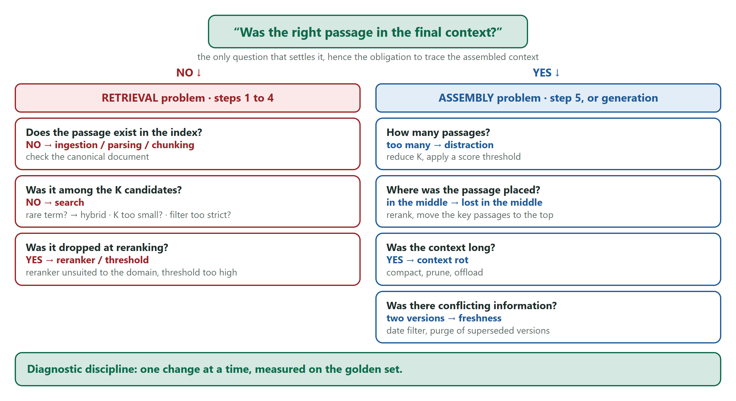
If the answer is no, the problem is upstream, steps 1 to 4, and each branch points at a precise component. If the answer is yes, it is assembly or generation. The diagnosis mirrors the structure of construction, which is the point of having walked the chain in order.

The methodological constraint: one change at a time, evaluated on the golden set. Simultaneous changes make the effect unattributable. It is what separates a team that progresses from a team that goes in circles. Five contracts to freeze early, so that an implementation can change without touching the rest: the canonical document, the chunk record (versioned JSONL), the retriever interface, the tool contract, and the assembled context object.

The proposed sequencing

Four waves, arbitrable from the golden set built in wave 1.

Wave	Content	Why
1 · The foundation, non-negotiable	Markdown normalisation · deduplication · structural chunking · metadata and access control · hybrid search · the golden set	Without these, neither measurement nor security is possible. They concentrate most of the gain.
2 · Short-term gains	Reranking and top-k calibration · system prompt and tool contract · prompt caching · compaction · tool index	The last three reduce cost while improving quality, which is rare and justifies treating them early.
3 · Deepening	Contextual Retrieval · sentence windows and parent-document · HyDE · memory · skills · int8 quantization	Arbitrable only from the golden set of wave 1.
4 · Specialisation	Late interaction and ColPali · graph (start with the document graph) · section tree · text-to-SQL · sub-agents · semantic cache	Triggered by a qualified need. Each one is a separate project.

Cross-cutting from wave 1: access control at the chunk, trust zones, the trifecta review. Structuring, not additive. Two deliverables: a reference architecture (pipeline diagram, metadata schema, need-to-architecture matrix) and a methodology (context template, tool-contract standard, memory and compaction policies).

Seven things to keep

Formulated as criteria that apply to other projects, not as conclusions specific to this one.

1. A model has only one input: the question is always what you put in it.
2. The context is not storage: past a threshold, adding degrades.
3. The quality ceiling is set at parsing; no downstream component raises it.
4. The search unit and the reading unit can be decoupled.
5. Dense and lexical have disjoint failure modes, hence hybrid by default.
6. Before choosing a RAG variant, check that a RAG is the answer.
7. Without a golden set and a trace of the assembled context, no decision can be arbitrated.

The sixth is the one that saves the most time in a workshop: in the matrix of step 4, a third of use cases do not call for a RAG. And the two deliverables to protect in wave 1 are the golden set and the trace of the assembled context.

Primary references

Every figure quoted above points to one of these sources.

Subject	Reference	Publication
Lost in the middle	Liu et al., "Lost in the Middle", arXiv:2307.03172	TACL 2024
Context rot	Hong, Troynikov, Huber, Chroma Research	July 2025
Parsing benchmark	OmniDocBench, OpenDataLab	CVPR 2025
Contextual Retrieval	Anthropic, "Introducing Contextual Retrieval"	September 2024
Summary hierarchy	Sarthi et al., RAPTOR	ICLR 2024
Deduplication	Broder, MinHash · Milvus MinHash-LSH index	1997 · 2025
Lexical weighting	Robertson and Zaragoza, Okapi BM25	2009
List fusion	Cormack, Clarke, Büttcher, Reciprocal Rank Fusion	SIGIR 2009
Late interaction	Khattab and Zaharia, ColBERT · Santhanam et al., ColBERTv2	NAACL 2022
Visual retrieval	Faysse et al., ColPali	2024
Knowledge graph	Edge et al., arXiv:2404.16130	Microsoft, April 2024
On-demand graph	Microsoft Research, LazyGraphRAG	June 2025
Text-to-SQL	Spider 1.0 · BIRD · Spider 2.0 · CHASE-SQL	2018 to 2025
Context engineering	Anthropic, "Effective context engineering for AI agents"	September 2025
CAG	Chan, Chen, Cheng, Huang, "Don't Do RAG", arXiv:2412.15605	December 2024
Tools and protocol	MCP (November 2024) · Agent Skills (October 2025) · Code execution with MCP	2024 to 2025
Prompt compression	LLMLingua · LLMLingua-2 · LongLLMLingua	EMNLP 2023 · ACL 2024
Agent memory	mem0 (arXiv:2504.19413, ECAI 2025) · Zep and Graphiti	2025
Multi-agent	Anthropic, "How we built our multi-agent research system"	June 2025
Security	OWASP Top 10 for LLM Applications · Willison, the lethal trifecta	2025

How much to trust the numbers

Not every figure above has the same status. The rule of citation: give the source and the date. A figure without provenance turns against whoever advances it.

Figure	Status	What it implies
Contextual Retrieval: −35 / −49 / −67 %	Primary source	Citable, with the mention Anthropic 2024
Lost in the middle: 75.8 / 53.8 / 56.1 %	Primary source	Specify GPT-3.5-Turbo and 20 passages
Context rot: breaks at 300 to 400k tokens	Primary source	18 models tested, July 2025
Multi-agent: +90.2 % and ×15 tokens	Primary source	Internal evaluation, not a public benchmark
LazyGraphRAG: 0.1 % of the indexing cost	Official announcement	No peer-reviewed publication
LongLLMLingua: +21.4 % at about 4× fewer tokens	Primary source	Measured on NaturalQuestions
GraphRAG: 879 vs 331,000 tokens per query	Primary paper, third-party costs	The paper is solid, the dollar figures are not
Prompt caching prices	Secondary sources	Re-check before any business case
Memory benchmarks (84 / 58 / 75 %)	Contested between vendors	Directional, never a selection criterion
OmniDocBench scores above 94 %	Saturated benchmark	Measure on your own documents
Binary quantization: 0.672 → 0.98	Vendor blog, reproducible	The protocol is described, the figures verifiable
MTEB ranks	Not comparable across versions	Version 2 changed the reference set
Semantic cache hit rates	Field reports	Depend on the traffic profile

If you keep one habit from this guide, make it the seventh takeaway: build the golden set in the first wave, record the assembled context on every query, and change one thing at a time. Everything else in the chain becomes arbitrable once those two artefacts exist.